TEB轨迹规划算法教程-优化反馈

TEB轨迹规划算法教程-优化反馈

说明：

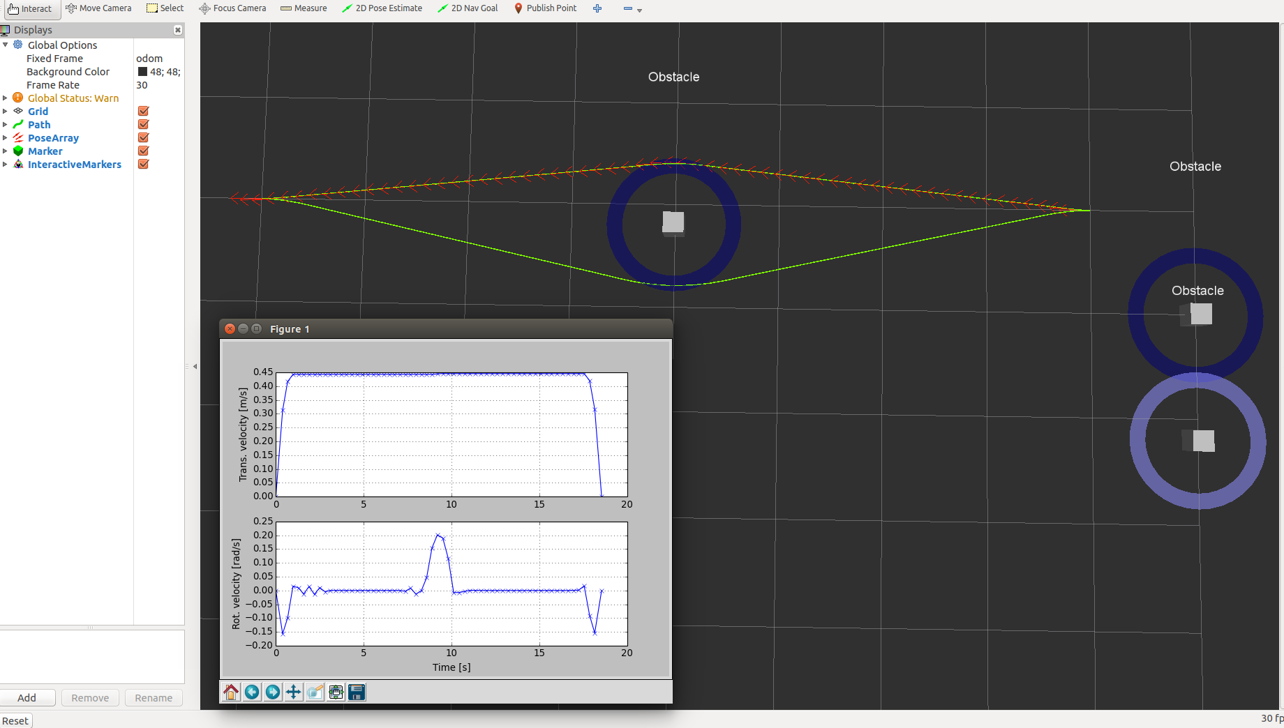
• 介绍如何检查优化轨迹的反馈; 提供了一个示例，其可视化当前所选轨迹的速度分布
• 在前面的示例中，您学习了如何测试优化，如何调整参数以及如何在rviz中可视化生成的轨迹。
• 然而，在rviz中可视化的轨迹不包含任何时间信息，仅显示其空间状态。
• 为了进一步参数调整或评估目的，可能有兴趣获得对底层优化状态的访问（涉及时间优化状态）。
• 因此teb_local_planner提供反馈消息teb_local_planner/FeedbackMsg，其包含所有内部状态和一些推断变量（如速度曲线）。
• 请注意，加速度曲线当前为空。
• 此外，该消息包含在独特拓扑中找到的所有备选轨迹。
• 当前选择的轨迹索引存储在变量selected_trajectory_idx中。
• 反馈主题（参见规划器API）可以由任何节点订阅（例如，将数据导出到文件，编写一些自定义可视化，......）。

注意：

• 默认情况下关闭发送反馈消息以减轻计算负担。
• 可以通过将rosparam ~/publish_feedback设置为true或通过调用rqt_reconfigure来启用它。

可视化速度曲线

• 在下文中，提供了一个小的python脚本，它订阅了上一个教程中介绍的test_optim_node。
• 脚本取决于pypose以创建绘图。
• 仅显示当前所选轨迹的速度分布。
• 脚本如下：

#!/usr/bin/env python

import rospy, math
from teb_local_planner.msg import FeedbackMsg, TrajectoryMsg, TrajectoryPointMsg
from geometry_msgs.msg import PolygonStamped, Point32
import numpy as np
import matplotlib.pyplot as plotter

def feedback_callback(data):
  global trajectory

  if not data.trajectories: # empty
    trajectory = []
    return
  trajectory = data.trajectories[data.selected_trajectory_idx].trajectory
  
  
def plot_velocity_profile(fig, ax_v, ax_omega, t, v, omega):
  ax_v.cla()
  ax_v.grid()
  ax_v.set_ylabel('Trans. velocity [m/s]')
  ax_v.plot(t, v, '-bx')
  ax_omega.cla()
  ax_omega.grid()
  ax_omega.set_ylabel('Rot. velocity [rad/s]')
  ax_omega.set_xlabel('Time [s]')
  ax_omega.plot(t, omega, '-bx')
  fig.canvas.draw()

  
  
def velocity_plotter():
  global trajectory
  rospy.init_node("visualize_velocity_profile", anonymous=True)
  
  topic_name = "/test_optim_node/teb_feedback" # define feedback topic here!
  rospy.Subscriber(topic_name, FeedbackMsg, feedback_callback, queue_size = 1) 

  rospy.loginfo("Visualizing velocity profile published on '%s'.",topic_name) 
  rospy.loginfo("Make sure to enable rosparam 'publish_feedback' in the teb_local_planner.")

  # two subplots sharing the same t axis
  fig, (ax_v, ax_omega) = plotter.subplots(2, sharex=True)
  plotter.ion()
  plotter.show()
  

  r = rospy.Rate(2) # define rate here
  while not rospy.is_shutdown():
    
    t = []
    v = []
    omega = []
    
    for point in trajectory:
      t.append(point.time_from_start.to_sec())
      v.append(point.velocity.linear.x)
      omega.append(point.velocity.angular.z)
          
    plot_velocity_profile(fig, ax_v, ax_omega, np.asarray(t), np.asarray(v), np.asarray(omega))
        
    r.sleep()

if __name__ == '__main__': 
  try:
    trajectory = []
    velocity_plotter()
  except rospy.ROSInterruptException:
    pass

• 该脚本已作为visualize_velocity_profile.py包含在teb_local_planner_tutorials包中。
• 假设roscore已经运行，可以将速度可视化如下：

rosparam set /test_optim_node/publish_feedback true # or use rqt_reconfigure later
roslaunch teb_local_planner test_optim_node.launch
rosrun teb_local_planner_tutorials visualize_velocity_profile.py # or call your own script here

• 您应该能够在运行时检查速度曲线，如下图所示：