


PythonRobotics机器人算法库-激光雷达栅格地图
纠错,疑问,交流: 请进入讨论区或 请点击进入页面,扫码加入微信群或Q群进行交流
获取最新文章: 扫一扫加入“创客智造”公众号
说明:
-
介绍如何从文件中读取 LIDAR(范围)测量值并将其转换为占用网格
步骤:
-
占用网格图(Hans Moravec,AE Elfes:High resolution maps from wide angle sonar,Proc. IEEE Int. Conf. Robotics Autom. (1985))是一种流行的概率方法来表示环境。
-
网格基本上是环境的离散表示,它显示网格单元是否被占用。这里的地图表示为 a ,接近 1 的数字表示该单元格已被占用(在下一张图像中用红色标记),接近 0 的数字表示它们空闲(用绿色标记)。
-
网格具有表示未知(未观察到)区域的能力,接近 0.5。

- 为了从测量中构建网格图,我们需要离散化这些值。但是,首先让我们需要import一些必要的包。
import math
import numpy as np
import matplotlib.pyplot as plt
from math import cos, sin, radians, pi- 测量文件包含距离和相应的角度csv(逗号分隔值)格式。让我们编写 file_read方法:
def file_read(f):
"""
Reading LIDAR laser beams (angles and corresponding distance data)
"""
measures = [line.split(",") for line in open(f)]
angles = []
distances = []
for measure in measures:
    angles.append(float(measure[0]))
    distances.append(float(measure[1]))
angles = np.array(angles)
distances = np.array(distances)
return angles, distances- 距离和角度可以很容易地用和确定x和 y坐标。为了显示它, 使用了matplotlib.pyplot (plt)
ang, dist = file_read("lidar01.csv")
ox = np.sin(ang) * dist
oy = np.cos(ang) * dist
plt.figure(figsize=(6,10))
plt.plot([oy, np.zeros(np.size(oy))], [ox, np.zeros(np.size(oy))], "ro-") # lines from 0,0 to the
plt.axis("equal")
bottom, top = plt.ylim()  # return the current ylim
plt.ylim((top, bottom)) # rescale y axis, to match the grid orientation
plt.grid(True)
plt.show()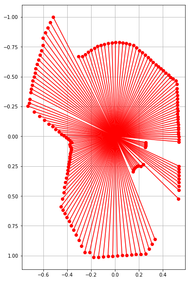
- 包含方便的lidar_to_grid_map.py函数,可用于将 2D 范围测量转换为网格图。例如, bresenham给出了网格图中两点之间的直线。让我们看看这是如何工作的
import lidar_to_grid_map as lg
map1 = np.ones((50, 50)) * 0.5
line = lg.bresenham((2, 2), (40, 30))
for l in line:
    map1[l[0]][l[1]] = 1
plt.imshow(map1)
plt.colorbar()
plt.show()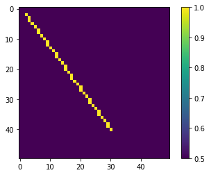
line = lg.bresenham((2, 30), (40, 30))
for l in line:
    map1[l[0]][l[1]] = 1
line = lg.bresenham((2, 30), (2, 2))
for l in line:
    map1[l[0]][l[1]] = 1
plt.imshow(map1)
plt.colorbar()
plt.show()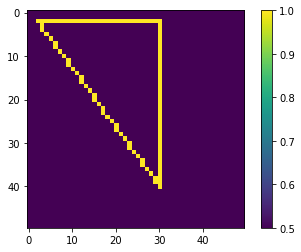
- 要填充空白区域,可以使用基于队列的算法,该算法可用于已初始化的占用图。给定中心点:算法在每次迭代中检查相邻元素,并停止在障碍物和自由边界上扩展
from collections import deque
def flood_fill(cpoint, pmap):
    """
    cpoint: starting point (x,y) of fill
    pmap: occupancy map generated from Bresenham ray-tracing
    """
    # Fill empty areas with queue method
    sx, sy = pmap.shape
    fringe = deque()
    fringe.appendleft(cpoint)
    while fringe:
        n = fringe.pop()
        nx, ny = n
        # West
        if nx > 0:
            if pmap[nx - 1, ny] == 0.5:
                pmap[nx - 1, ny] = 0.0
                fringe.appendleft((nx - 1, ny))
        # East
        if nx < sx - 1:
            if pmap[nx + 1, ny] == 0.5:
                pmap[nx + 1, ny] = 0.0
                fringe.appendleft((nx + 1, ny))
        # North
        if ny > 0:
            if pmap[nx, ny - 1] == 0.5:
                pmap[nx, ny - 1] = 0.0
                fringe.appendleft((nx, ny - 1))
        # South
        if ny < sy - 1:
            if pmap[nx, ny + 1] == 0.5:
                pmap[nx, ny + 1] = 0.0
fringe.appendleft((nx, ny + 1))- 该算法将从中心点(例如 (10, 20))开始用零填充由黄线界定的区域:
flood_fill((10, 20), map1)
map_float = np.array(map1)/10.0
plt.imshow(map1)
plt.colorbar()
plt.show()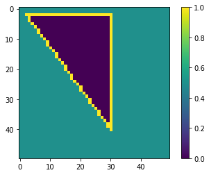
- 让我们对真实数据使用flood填充:
xyreso = 0.02  # x-y grid resolution
yawreso = math.radians(3.1)  # yaw angle resolution [rad]
ang, dist = file_read("lidar01.csv")
ox = np.sin(ang) * dist
oy = np.cos(ang) * dist
pmap, minx, maxx, miny, maxy, xyreso = lg.generate_ray_casting_grid_map(ox, oy, xyreso, False)
xyres = np.array(pmap).shape
plt.figure(figsize=(20,8))
plt.subplot(122)
plt.imshow(pmap, cmap = "PiYG_r")
plt.clim(-0.4, 1.4)
plt.gca().set_xticks(np.arange(-.5, xyres[1], 1), minor = True)
plt.gca().set_yticks(np.arange(-.5, xyres[0], 1), minor = True)
plt.grid(True, which="minor", color="w", linewidth = .6, alpha = 0.5)
plt.colorbar()
plt.show()-
进入目录PythonRobotics/Mapping/lidar_to_grid_map
-
执行文件
python3 lidar_to_grid_map.py- 结果如下
The grid map is 150 x 100 .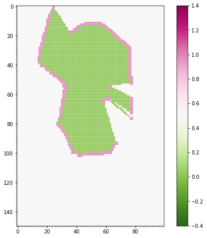
纠错,疑问,交流: 请进入讨论区或 请点击进入页面,扫码加入微信群或Q群进行交流
获取最新文章: 扫一扫加入“创客智造”公众号