


PythonRobotics机器人算法库-Graph based SLAM
纠错,疑问,交流: 请进入讨论区或 请点击进入页面,扫码加入微信群或Q群进行交流
获取最新文章: 扫一扫加入“创客智造”公众号
说明:
-
这是一个基于Graph SLAM的示例
介绍:
- Graph SLAM
import copy
import math
import itertools
import numpy as np
import matplotlib.pyplot as plt
from graph_based_slam import calc_rotational_matrix, calc_jacobian, cal_observation_sigma, \
                             calc_input, observation, motion_model, Edge, pi_2_pi

%matplotlib inline
np.set_printoptions(precision=3, suppress=True)
np.random.seed(0)-
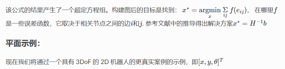
与解决 SLAM 的概率方法(例如 EKF、UKF、粒子滤波器等)相比,图技术将 SLAM 表述为优化问题。它主要用于以离线方式解决完整的 SLAM 问题,即在遍历路径后优化机器人的所有姿势。然而,一些变体可用,它们使用基于图形的方法来执行在线估计或求解姿势的子集
-
GraphSLAM 使用运动信息以及对环境的观察来创建可以使用标准优化技术解决的最小二乘问题

R = 0.2
Q = 0.2
N = 3
graphics_radius = 0.1

odom = np.empty((N,1))
obs = np.empty((N,1))
x_true = np.empty((N,1))

landmark = 3
# Simulated readings of odometry and observations
x_true[0], odom[0], obs[0] = 0.0, 0.0, 2.9
x_true[1], odom[1], obs[1] = 1.0, 1.5, 2.0
x_true[2], odom[2], obs[2] = 2.0, 2.4, 1.0

hxDR = copy.deepcopy(odom)
# Visualization
plt.plot(landmark,0, '*k', markersize=30)
for i in range(N):
    plt.plot(odom[i], 0, '.', markersize=50, alpha=0.8, color='steelblue')
    plt.plot([odom[i], odom[i] + graphics_radius],
             [0,0], 'r')
    plt.text(odom[i], 0.02, "X_{}".format(i), fontsize=12)
    plt.plot(obs[i]+odom[i],0,'.', markersize=25, color='brown')
    plt.plot(x_true[i],0,'.g', markersize=20)
plt.grid()
plt.show()


# Defined as a function to facilitate iteration
def get_H_b(odom, obs):
    """
    Create the information matrix and information vector. This implementation is
    based on the concept of virtual measurement i.e. the observations of the
    landmarks are converted into constraints (edges) between the nodes that
    have observed this landmark.
    """
    measure_constraints = {}
    omegas = {}
    zids = list(itertools.combinations(range(N),2))
    H = np.zeros((N,N))
    b = np.zeros((N,1))
    for (t1, t2) in zids:
        x1 = odom[t1]
        x2 = odom[t2]
        z1 = obs[t1]
        z2 = obs[t2]

        # Adding virtual measurement constraint
        measure_constraints[(t1,t2)] = (x2-x1-z1+z2)
        omegas[(t1,t2)] = (1 / (2*Q))

        # populate system's information matrix and vector
        H[t1,t1] += omegas[(t1,t2)]
        H[t2,t2] += omegas[(t1,t2)]
        H[t2,t1] -= omegas[(t1,t2)]
        H[t1,t2] -= omegas[(t1,t2)]

        b[t1] += omegas[(t1,t2)] * measure_constraints[(t1,t2)]
        b[t2] -= omegas[(t1,t2)] * measure_constraints[(t1,t2)]

    return H, b


H, b = get_H_b(odom, obs)
print("The determinant of H: ", np.linalg.det(H))
H[0,0] += 1 # np.inf ?
print("The determinant of H after anchoring constraint: ", np.linalg.det(H))

for i in range(5):
    H, b = get_H_b(odom, obs)
    H[(0,0)] += 1

    # Recover the posterior over the path
    dx = np.linalg.inv(H) @ b
    odom += dx
    # repeat till convergence
print("Running graphSLAM ...")
print("Odometry values after optimzation: \n", odom)

plt.figure()
plt.plot(x_true, np.zeros(x_true.shape), '.', markersize=20, label='Ground truth')
plt.plot(odom, np.zeros(x_true.shape), '.', markersize=20, label='Estimation')
plt.plot(hxDR, np.zeros(x_true.shape), '.', markersize=20, label='Odom')
plt.legend()
plt.grid()
plt.show()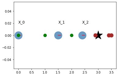
The determinant of H:  0.0
The determinant of H after anchoring constraint:  18.750000000000007
Running graphSLAM ...
Odometry values after optimzation:
 [[-0. ]
 [ 0.9]
 [ 1.9]]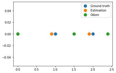

#  Simulation parameter
Qsim = np.diag([0.01, np.deg2rad(0.010)])**2 # error added to range and bearing
Rsim = np.diag([0.1, np.deg2rad(1.0)])**2 # error added to [v, w]

DT = 2.0  # time tick [s]
SIM_TIME = 100.0  # simulation time [s]
MAX_RANGE = 30.0  # maximum observation range
STATE_SIZE = 3  # State size [x,y,yaw]

# TODO: Why not use Qsim ?
# Covariance parameter of Graph Based SLAM
C_SIGMA1 = 0.1
C_SIGMA2 = 0.1
C_SIGMA3 = np.deg2rad(1.0)

MAX_ITR = 20  # Maximum iteration during optimization
timesteps = 1

# consider only 2 landmarks for simplicity
# RFID positions [x, y, yaw]
RFID = np.array([[10.0, -2.0, 0.0],
#                  [15.0, 10.0, 0.0],
#                  [3.0, 15.0, 0.0],
#                  [-5.0, 20.0, 0.0],
#                  [-5.0, 5.0, 0.0]
                 ])

# State Vector [x y yaw v]'
xTrue = np.zeros((STATE_SIZE, 1))
xDR = np.zeros((STATE_SIZE, 1))  # Dead reckoning
xTrue[2] = np.deg2rad(45)
xDR[2] = np.deg2rad(45)
# history initial values
hxTrue = xTrue
hxDR = xTrue
_, z, _, _ = observation(xTrue, xDR, np.array([[0,0]]).T, RFID)
hz = [z]

for i in range(timesteps):
    u = calc_input()
    xTrue, z, xDR, ud = observation(xTrue, xDR, u, RFID)
    hxDR = np.hstack((hxDR, xDR))
    hxTrue = np.hstack((hxTrue, xTrue))
    hz.append(z)

# visualize
graphics_radius = 0.3
plt.plot(RFID[:, 0], RFID[:, 1], "*k", markersize=20)
plt.plot(hxDR[0, :], hxDR[1, :], '.', markersize=50, alpha=0.8, label='Odom')
plt.plot(hxTrue[0, :], hxTrue[1, :], '.', markersize=20, alpha=0.6, label='X_true')

for i in range(hxDR.shape[1]):
    x = hxDR[0, i]
    y = hxDR[1, i]
    yaw = hxDR[2, i]
    plt.plot([x, x + graphics_radius * np.cos(yaw)],
             [y, y + graphics_radius * np.sin(yaw)], 'r')
    d = hz[i][:, 0]
    angle = hz[i][:, 1]
    plt.plot([x + d * np.cos(angle + yaw)], [y + d * np.sin(angle + yaw)], '.',
             markersize=20, alpha=0.7)
    plt.legend()
plt.grid()
plt.show()
# Copy the data to have a consistent naming with the .py file
zlist = copy.deepcopy(hz)
x_opt = copy.deepcopy(hxDR)
xlist = copy.deepcopy(hxDR)
number_of_nodes = x_opt.shape[1]
n = number_of_nodes * STATE_SIZE- 保存数据后,将通过查看每对节点来构建图形。仅当两个节点在不同时间点观察到相同地标时,才会创建虚拟测量。下一个单元格是图构造-> 优化-> 估计更新的单次迭代的演练。
# get all the possible combination of the different node
zids = list(itertools.combinations(range(len(zlist)), 2))
print("Node combinations: \n", zids)

for i in range(xlist.shape[1]):
    print("Node {} observed landmark with ID {}".format(i, zlist[i][0, 3]))


Node combinations:
 [(0, 1)]
Node 0 observed landmark with ID 0.0
Node 1 observed landmark with ID 0.0-
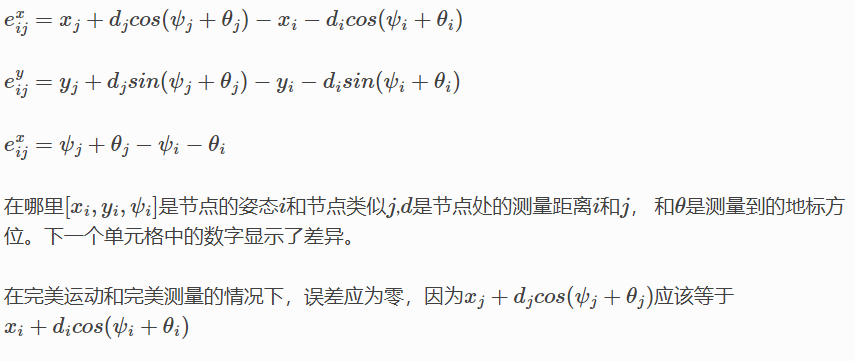
在以下代码片段中,将创建基于节点 0 和 1 之间的虚拟测量的错误。误差方程如下:
-
# Initialize edges list
edges = []

# Go through all the different combinations
for (t1, t2) in zids:
    x1, y1, yaw1 = xlist[0, t1], xlist[1, t1], xlist[2, t1]
    x2, y2, yaw2 = xlist[0, t2], xlist[1, t2], xlist[2, t2]

    # All nodes have valid observation with ID=0, therefore, no data association condition
    iz1 = 0
    iz2 = 0

    d1 = zlist[t1][iz1, 0]
    angle1, phi1 = zlist[t1][iz1, 1], zlist[t1][iz1, 2]
    d2 = zlist[t2][iz2, 0]
    angle2, phi2 = zlist[t2][iz2, 1], zlist[t2][iz2, 2]

    # find angle between observation and horizontal
    tangle1 = pi_2_pi(yaw1 + angle1)
    tangle2 = pi_2_pi(yaw2 + angle2)

    # project the observations
    tmp1 = d1 * math.cos(tangle1)
    tmp2 = d2 * math.cos(tangle2)
    tmp3 = d1 * math.sin(tangle1)
    tmp4 = d2 * math.sin(tangle2)

    edge = Edge()
    print(y1,y2, tmp3, tmp4)
    # calculate the error of the virtual measurement
    # node 1 as seen from node 2 throught the observations 1,2
    edge.e[0, 0] = x2 - x1 - tmp1 + tmp2
    edge.e[1, 0] = y2 - y1 - tmp3 + tmp4
    edge.e[2, 0] = pi_2_pi(yaw2 - yaw1 - tangle1 + tangle2)

    edge.d1, edge.d2 = d1, d2
    edge.yaw1, edge.yaw2 = yaw1, yaw2
    edge.angle1, edge.angle2 = angle1, angle2
    edge.id1, edge.id2 = t1, t2

    edges.append(edge)

    print("For nodes",(t1,t2))
    print("Added edge with errors: \n", edge.e)

    # Visualize measurement projections
    plt.plot(RFID[0, 0], RFID[0, 1], "*k", markersize=20)
    plt.plot([x1,x2],[y1,y2], '.', markersize=50, alpha=0.8)
    plt.plot([x1, x1 + graphics_radius * np.cos(yaw1)],
             [y1, y1 + graphics_radius * np.sin(yaw1)], 'r')
    plt.plot([x2, x2 + graphics_radius * np.cos(yaw2)],
             [y2, y2 + graphics_radius * np.sin(yaw2)], 'r')

    plt.plot([x1,x1+tmp1], [y1,y1], label="obs 1 x")
    plt.plot([x2,x2+tmp2], [y2,y2], label="obs 2 x")
    plt.plot([x1,x1], [y1,y1+tmp3], label="obs 1 y")
    plt.plot([x2,x2], [y2,y2+tmp4], label="obs 2 y")
    plt.plot(x1+tmp1, y1+tmp3, 'o')
    plt.plot(x2+tmp2, y2+tmp4, 'o')
plt.legend()
plt.grid()
plt.show()


0.0 1.427649841628278 -2.0126109674819155 -3.524048014922737
For nodes (0, 1)
Added edge with errors:
 [[-0.02 ]
 [-0.084]
 [ 0.   ]]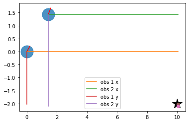

# Initialize the system information matrix and information vector
H = np.zeros((n, n))
b = np.zeros((n, 1))
x_opt = copy.deepcopy(hxDR)

for edge in edges:
    id1 = edge.id1 * STATE_SIZE
    id2 = edge.id2 * STATE_SIZE

    t1 = edge.yaw1 + edge.angle1
    A = np.array([[-1.0, 0, edge.d1 * math.sin(t1)],
                  [0, -1.0, -edge.d1 * math.cos(t1)],
                  [0, 0, -1.0]])

    t2 = edge.yaw2 + edge.angle2
    B = np.array([[1.0, 0, -edge.d2 * math.sin(t2)],
                  [0, 1.0, edge.d2 * math.cos(t2)],
                  [0, 0, 1.0]])

    # TODO: use Qsim instead of sigma
    sigma = np.diag([C_SIGMA1, C_SIGMA2, C_SIGMA3])
    Rt1 = calc_rotational_matrix(tangle1)
    Rt2 = calc_rotational_matrix(tangle2)
    edge.omega = np.linalg.inv(Rt1 @ sigma @ Rt1.T + Rt2 @ sigma @ Rt2.T)

    # Fill in entries in H and b
    H[id1:id1 + STATE_SIZE, id1:id1 + STATE_SIZE] += A.T @ edge.omega @ A
    H[id1:id1 + STATE_SIZE, id2:id2 + STATE_SIZE] += A.T @ edge.omega @ B
    H[id2:id2 + STATE_SIZE, id1:id1 + STATE_SIZE] += B.T @ edge.omega @ A
    H[id2:id2 + STATE_SIZE, id2:id2 + STATE_SIZE] += B.T @ edge.omega @ B

    b[id1:id1 + STATE_SIZE] += (A.T @ edge.omega @ edge.e)
    b[id2:id2 + STATE_SIZE] += (B.T @ edge.omega @ edge.e)


print("The determinant of H: ", np.linalg.det(H))
plt.figure()
plt.subplot(1,2,1)
plt.imshow(H, extent=[0, n, 0, n])
plt.subplot(1,2,2)
plt.imshow(b, extent=[0, 1, 0, n])
plt.show()

# Fix the origin, multiply by large number gives same results but better visualization
H[0:STATE_SIZE, 0:STATE_SIZE] += np.identity(STATE_SIZE)
print("The determinant of H after origin constraint: ", np.linalg.det(H))
plt.figure()
plt.subplot(1,2,1)
plt.imshow(H, extent=[0, n, 0, n])
plt.subplot(1,2,2)
plt.imshow(b, extent=[0, 1, 0, n])
plt.show()


The determinant of H:  0.0
The determinant of H after origin constraint:  716.1972439134893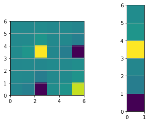
# Find the solution (first iteration)
dx = - np.linalg.inv(H) @ b
for i in range(number_of_nodes):
    x_opt[0:3, i] += dx[i * 3:i * 3 + 3, 0]
print("dx: \n",dx)
print("ground truth: \n ",hxTrue)
print("Odom: \n", hxDR)
print("SLAM: \n", x_opt)

# performance will improve with more iterations, nodes and landmarks.
print("\ngraphSLAM localization error: ", np.sum((x_opt - hxTrue) ** 2))
print("Odom localization error: ", np.sum((hxDR - hxTrue) ** 2))


dx:
 [[-0.   ]
 [-0.   ]
 [ 0.   ]
 [ 0.02 ]
 [ 0.084]
 [-0.   ]]
ground truth:
  [[0.    1.414]
 [0.    1.414]
 [0.785 0.985]]
Odom:
 [[0.    1.428]
 [0.    1.428]
 [0.785 0.976]]
SLAM:
 [[-0.     1.448]
 [-0.     1.512]
 [ 0.785  0.976]]

graphSLAM localization error:  0.010729072751057656
Odom localization error: 0.0004460978857535104-
进入目录/PythonRobotics/SLAM/GraphBasedSLAM
-
执行文件
python3 graph_based_slam.py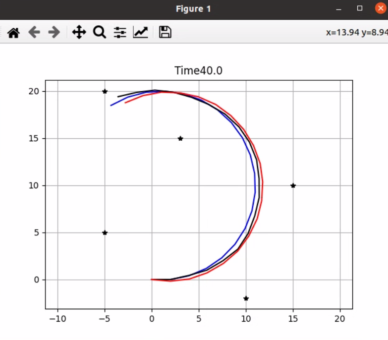
- 结果如下
graph_based_slam.py start!!
start graph based slam
cost: 29953.271102707055 ,n_edge: 225
iteration: 1, diff: 2.111720
cost: 34.482997286800064 ,n_edge: 225
iteration: 2, diff: 0.180774
cost: 17.69751656593137 ,n_edge: 225
iteration: 3, diff: 0.008879
cost: 17.693679702827733 ,n_edge: 225
iteration: 4, diff: 0.000593
cost: 17.69363144483148 ,n_edge: 225
iteration: 5, diff: 0.000040
cost: 17.693629175812728 ,n_edge: 225
iteration: 6, diff: 0.000003
start graph based slam
cost: 351002.29789791146 ,n_edge: 950
iteration: 1, diff: 26.350800
cost: 1062.3405915726482 ,n_edge: 950
iteration: 2, diff: 2.681332
cost: 101.25746059274898 ,n_edge: 950
iteration: 3, diff: 0.064795
cost: 100.68132888668202 ,n_edge: 950
iteration: 4, diff: 0.001667
cost: 100.68075185139209 ,n_edge: 950
iteration: 5, diff: 0.000043
cost: 100.68074665640461 ,n_edge: 950
iteration: 6, diff: 0.000001
start graph based slam
cost: 1011950.7444878097 ,n_edge: 2175
iteration: 1, diff: 97.553762
cost: 2453.4998048622074 ,n_edge: 2175
iteration: 2, diff: 2.393300
cost: 222.1900284805346 ,n_edge: 2175
iteration: 3, diff: 0.049059
cost: 221.44028268317817 ,n_edge: 2175
iteration: 4, diff: 0.001021
cost: 221.4397369533094 ,n_edge: 2175
iteration: 5, diff: 0.000021
cost: 221.43973238759688 ,n_edge: 2175
iteration: 6, diff: 0.000000
start graph based slam
cost: 1769808.7799064808 ,n_edge: 3900
iteration: 1, diff: 230.044247
cost: 3838.394100244781 ,n_edge: 3900
iteration: 2, diff: 1.204398
cost: 431.50235998593905 ,n_edge: 3900
iteration: 3, diff: 0.026817
cost: 431.3135140349668 ,n_edge: 3900
iteration: 4, diff: 0.000743
cost: 431.3131409373172 ,n_edge: 3900
iteration: 5, diff: 0.000021
cost: 431.31313444416287 ,n_edge: 3900
iteration: 6, diff: 0.000001
start graph based slam
cost: 2736633.37849904 ,n_edge: 6125
iteration: 1, diff: 379.514143
cost: 4939.791622796388 ,n_edge: 6125
iteration: 2, diff: 0.912985
cost: 702.2442105157007 ,n_edge: 6125
iteration: 3, diff: 0.014780
cost: 702.1842574827197 ,n_edge: 6125
iteration: 4, diff: 0.000342
cost: 702.1840993083136 ,n_edge: 6125
iteration: 5, diff: 0.000008
纠错,疑问,交流: 请进入讨论区或 请点击进入页面,扫码加入微信群或Q群进行交流
获取最新文章: 扫一扫加入“创客智造”公众号